A Simple Rating System for Staffing Graph Projects
A business unit leader once asked me a simple question: When will my development team be self-sufficient in creating graph applications? Although the question was simple, my answer required the business leader to understand two concepts. The first was measuring graph developers’ proficiency and skill level. The second was understanding how a development team needs a mix of developers with various skill levels.
This blog will cover both of these concepts. It will also help you design a team structure with the right mix and know when to supplement your team with outside experts.
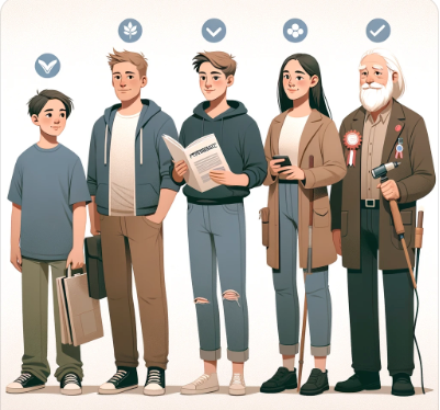
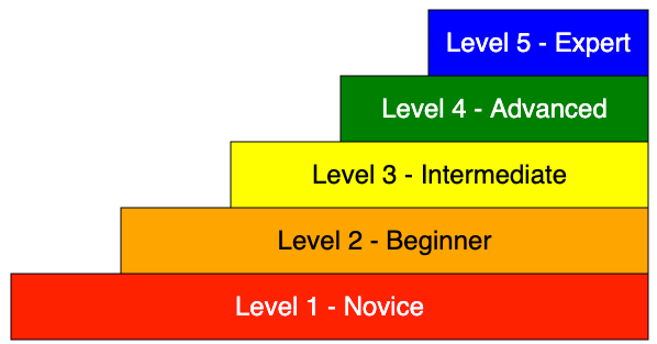
As any team gains experience with graph databases, it is expected to ask, “What is the overall level of proficiency my development team has?” We can answer this question by assigning each member of the team a graph proficiency rating. It is a numeric score that ranges from level 1 (Novice) to level 5 (Expert). Note that this ranking is ONLY for the graph developer persona. A separate proficiency rating is used for operations teams.
When any new TigerGraph project starts, a team of TigerGraph experts can assess your team’s skill level. This assessment can estimate the amount of professional services you will need for the initial phases of your project while your internal teams get up to speed.
This diagram allows you to hover over each level, and the description will be displayed below the diagram.
Here is our suggested ranking system.
Level 1: Novice
At the novice level, individuals have a basic understanding of graph databases learning basic terminology, such as when to use vertices, edges, and attributes. They understand concepts such as directed edges and basic graph traversal. Novice graph developers have begun to have experience designing simple graph models of up to about a dozen vertices. They can perform basic read operations, call building queries, and write or modify simple GSQL. They struggle with complex query syntax and logic. Novices rely heavily on their peers and need clear examples, documentation, and significant guidance and supervision.
Estimated Time to Achieve Novice Proficiency: 1-2 months.
Level 2: Beginner
Beginners understand fundamental graph database concepts and can design more complicated graph data models with some guidance. They are starting to model relationships and attributes and write simple traversal queries in GSQL using essential functions and clauses. They begin to use accumulators to optimize queries. Beginners occasionally need help with syntax and logic and require moderate supervision and review. They are exposed to graph algorithms such as breadth-first search and PageRank. They can participate in graph development projects, but senior developers should review their code.
Estimated Time to Achieve: 2-5 months.
Level 3: Intermediate
At the intermediate level, individuals have a solid understanding of graph database principles and can independently design moderately complex graph models. They are proficient in writing more complex GSQL queries, including multi-step traversals, and are comfortable optimizing basic queries for performance. They have developed skills for debugging GSQL queries and leveraging a library of graph algorithms such as label propagation pathfinding and community detection. They can quickly come up to speed and contribute to various graph projects. They occasionally seek guidance on advanced query constructs and best practices.
Estimated Time to Achieve: 5-12 months.
Level 4: Advanced
Advanced practitioners understand graph database principles and can independently design complex and efficient graph models for diverse use cases. Advanced graph developers know design tradeoffs and can visualize memory allocation patterns used in vertex-attached accumulators. They are highly proficient in writing and optimizing complex GSQL queries, comfortable with advanced features, and can troubleshoot complex query issues. Advanced graph developers have real-world experience using a wide variety of graph algorithms. They get exposure to query optimization and can write User Defined Functions (UDFs) in low-level C code. Advanced individuals can mentor others and guide best practices and optimization.
Estimated Time to Achieve: 1-2 years.
Level 5: Expert
Experts deeply understand property graph databases and data modeling and can design highly complex, scalable, and efficient graph models. Experts master GSQL (or Cypher) and its advanced features and quickly write, optimize, and troubleshoot the most complicated queries. Experts act as subject matter experts, contributing to improving team knowledge through mentorship and training, and are seen as thought leaders within the organization. Experts lead the design of new graph projects and can quickly assess the proficiency level of their peers and accurately recommend training paths for junior developers. Expert users can also explain the benefits of graph databases to senior leadership and compare and contrast graph databases with other databases such as relational databases, analytical databases, key-value stores, column-family stores, and document stores. Experts can draw on a deep portfolio of stories and experiences of how graphs have been used to solve complex business problems.
Estimated Time to Achieve: 2+ years.
Getting the Mix Right
When you start any new project, you should have a healthy mixture of level 3, 4, and 5 staff. You may not need full-time level 5 expert staff, but you need some part-time staff available to perform code reviews and mentor junior staff. Sometimes, due to budget constraints, your team will consist mainly of 1s and 2s. Junior developers often need to be corrected and redesign systems, slowing their progress. The junior your team is, the more frequent your code review cycles should be.
Here is a typical mix for a new TigerGraph project:
3 Novices
2 Beginners
1 Intermediate
1 Advanced
¼ Time Expert
Here is an example of a project that had severe challenges reaching deadlines:
5 Novices
3 Beginners
¼ Time Intermediate
If this is a makeup of your team, consider adding professional services staff from TigerGraph until your staff has time to come up to speed.
Conclusion
Working with any new technology takes time and patience. With a TigerGraph Customer Success Plan, you can rest assured that we will bring our expertise to your team and maximize your odds of project success.
References
Several papers and websites contain information about measuring developer skills and go into some depth on its complexity and the process of measuring educational goals. These metrics are called Rubrics. This article leverages some of their terminology but applies it to graph developers.
The Rise of GQL: A New ISO Standard in Graph Query Language
We’re thrilled to celebrate a significant milestone in the world of database technology: the publication of the first version of the ISO GQL standard on April 12, 2024. You can access the standard here.
As an active contributor to the development of GQL standard version 1, I’ve witnessed the entire journey from its inception to its high-quality final publication. I can attest that this marks a significant milestone in the history of databases. Thanks to the GQL editor Stefan Plantikow and Stephen Cannan, editing tooling support from Jim Melton, the convenor of WG3 Keith Hare, and the original author of the GQL manifesto Alastair Green. This elegant standard is developed with a strong international team including both academia and industry query language experts. A non-exhaustive contributor list can be found on these two SIGMOD papers 1, 2.
In this blog, I’m going to share my personal enthusiasm on GQL and invite you to start learning it.
What is GQL?
GQL, or Graph Query Language, is an ISO standard defined for property graph databases. It stands as the first sibling database language emerging from the ISO standard committee for databases since the initial publication of the SQL standard in 1986.
GQL aims to become the de facto query language standard for property graph databases, addressing the growing demand for such databases.
Let’s revisit some background knowledge on property graph databases.
Firstly, property graph databases utilize property graph data modeling, where vertices and edges serve as the fundamental units to represent data elements. In contrast, the traditional relational data model relies on tables for data representation. Intuitively, the property graph model offers greater flexibility and aligns more closely with real-world interactions between objects.
Secondly, there are various storage formats tailored to support the property graph data model. Native graph databases distinguish themselves from non-native counterparts primarily through their storage format. In a native graph database, vertices and edges are treated as first-class citizens within the storage layer, resulting in superior performance, particularly in path traversal and iterative graph algorithms. This performance boost stems from the native graph database’s inherent structure as a gigantic object index. During graph traversal, one navigates from an active vertex set to another via their connecting edges, circumventing the need for costly runtime joins (as relational databases do) to reconnect data elements. In my opinion, native graph database’s graph storage format is the key differentiator to other databases. TigerGraph falls in the category of native graph database.
Why GQL and Why Now?
As the graph database industry evolves, it becomes the third canonical database, alongside relational databases and key-value store databases. In the past decade, the burgeoning graph database industry has witnessed a plethora of vendors offering their own graph database products, each accompanied by their proprietary graph query language. Examples include Neo4j’s Cypher, TigerGraph’s GSQL, Oracle’s PGQ, LDBC’s G-core, and Gremlin, among others. For a comprehensive overview of the graph query language landscape, I recommend referring to Peter Boncz’s insightful survey slide from CWI.
Amidst this thriving ecosystem, GQL emerged to address the growing demand for a standardized graph query language. Its publication establishes a solid foundation and drives the prosperity of graph databases in the coming years, akin to what SQL did for relational databases
Scratching the GQL Surface
At its core, GQL uses pattern matching syntax to declaratively ask queries against graph databases, similar to SQL for relational databases.
The building blocks of a pattern are (1) vertex pattern and (2) edge pattern, illustrated below.
MATCH (x:Account WHERE x.isBlocked=’no’)
x binds to a vertex in the graph. () is a node pattern.
MATCH −[e:Transfer WHERE e.amount>5M]−>
e binds to an edge in the graph. -[]-> is an edge pattern.
With the above building blocks, you can have a longer pattern by alternating the node and edge patterns.
MATCH (x:Account)-[:SignInWithIP]->(y:IP)
-[:Associated]->(p:Phone)
Each matched pattern provides a table. You can filter, group by, aggregate, and project the columns of the table, as you do in SQL.
GQL has two syntax flavors: one is Cypher, and the other is SQL. However, both flavors share the same core pattern matching part.
If you’re coming from the SQL world, you’ll use something like this.
SELECT x.age, y.ip FROM g MATCH (x:Account)-[:SignInWithIP]-(y:IP) WHERE x.name == “John”
Note: TigerGraph is the main contributor and advocate for the SQL flavor in GQL because we firmly believe that SQL users will have a much easier time learning GQL with the SQL dialect.
If you’re familiar with the Cypher world, you’ll use something like the example below.
MATCH (x:Account)-[:SignInWithIP]-(y:IP) WHERE x.name == “John” RETURN x.age, y.ip
Furthermore, GQL supports linear composition of pattern match statements, meaning that each MATCH statement’s generated result table columns can be used to drive the next MATCH statement. This linear composition can be illustrated by the two flavors:
SQL flavor
{
SELECT expression_list FROM g MATCH graph_pattern1 WHERE xxx
NEXT
SELECT expression_list FROM g MATCH graph_pattern2 WHERE yyy
NEXT
SELECT expression_list FROM g MATCH graph_pattern3 WHERE zzz
}
Cypher flavor
{
USE g MATCH graph_pattern1 WHERE xxx YIELD expression_list
NEXT
USE g MATCH graph_pattern2 WHERE yyy YIELD expression_list
NEXT
USE g MATCH graph_pattern2 WHERE zzz RETURN expression_list
}
Besides the query syntax, GQL also supports a Linux file system-style directory hierarchy to host graph schemas and their catalog objects. This physical design of the catalog layout is to adapt to the flexibility of two-level property graph modeling, where a graph is a logical container and vertices and edges are the base containers. This design was initially informally discussed between TigerGraph and Neo4j, as we were first inspired by our multi-graph modeling product offering—multiple graphs can share a subset of the base vertex and edge containers. After multi-round constructive discussions, we agree that graph schemas will evolve freely under this catalog layout, especially for cross graph sharing and joining.
There are many other gems in the GQL standard; interested readers can purchase and study the standard.
How To Learn It?
Many TigerGraph users have asked me how to learn GQL or have an early peek. Here is my suggested approach for a quick ramp-up:
Study the core pattern matching design: get familiar with the Pattern Match syntax by reading this SIGMOD paper. It lays the foundation for understanding pattern matching nuances and design philosophy.
Study existing LDBC-SNB BI benchmark queries written in Cypher and GSQL. They bear many similarities to GQL syntax.
Dive into the Standard: read the 628-page ISO GQL standard (cost: 217 CHF) for a comprehensive understanding of the language’s specifications.
Last and the most important thing, start writing!
What’s Next for GQL?
GQL version 1 marks just the beginning of an ongoing journey. As the industry evolves, there are still challenges to address, including graph view support, trigger support, enhanced graph algorithm capabilities, and join graphs and tables, among others. At TigerGraph, we’re actively implementing GQL to champion this standard, maintaining our unwavering commitment to both openCypher and GQL.
Reflecting on our journey, Alin Deutsch, Yu Xu, and I began inventing GSQL in the summer of 2015 in Mountain View, CA, drawing inspiration from both the SQL standard and pattern matching literature. Alin and I implemented the initial version of GSQL that summer, burning many night candles. Throughout this process, we’ve contributed our best practices and real-world experiences back to the ISO GQL standard. We’re continuing this journey with the ISO standard committee, actively shaping the future versions of GQL. Along the way, we’ve forged numerous friendships within the global graph community, collectively delivering this beautiful standard. We hope you’ll recognize the dedication and passion this community has poured into this endeavor and take the time to learn, appreciate the design, and, most importantly, start using it.
In conclusion, GQL represents a significant leap forward in standardizing graph query languages. Whether you’re a seasoned database professional or new to graph databases, now is the time to start learning GQL and embrace the future of graph data management. Stay tuned for exciting developments in the world of GQL!
If you want to learn more about TigerGraph and GQL contact us at info@tigergraph.abstage.xyz.
Graph embeddings have become increasingly important in Enterprise Knowledge Graph (EKG) strategy. Graph embeddings will soon become the de facto way to quickly find similar items in large billion-vertex EKGs. And as we have discussed in our prior articles, real-time similarity calculations are critical to many areas such as recommendation, next best action, and cohort building.
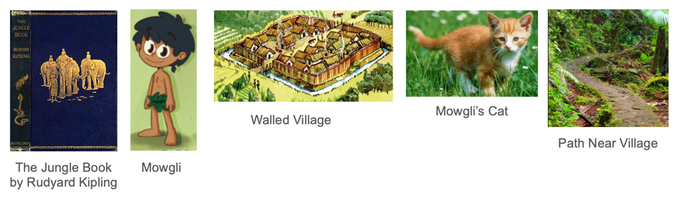
The goal of this article is to give you an intuitive feeling for what graph embeddings are and how they are used so you can decide if these are right for your EKG project. For those of you with a bit of data science background, we will also touch a bit on how they are calculated. For the most part, we will be using storytelling and metaphors to explain these concepts. We hope you can use these stories to explain graph embeddings to your non-technical peers in a fun and memorable way. Let’s start with our first story, which I call “Mowgli’s Walk.”
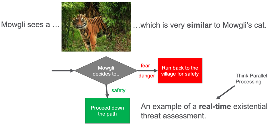
Mowgli is a young boy that lives in a prehistoric village with a sturdy protective wall around it. Mowgli has a cute pet cat with orange fur and stripes. One day, Mowgli walks down a path just outside the village wall and sees a large tiger in the path ahead. What should Mowgli do?
Mowgli sees a tiger on the path. What should he do? Run back to the village or proceed down the path.
Should he continue down the path or quickly run back to the village and the safety of the wall? Mowgli does not have a lot of time to make this decision. Perhaps only a few seconds. Mowgli’s brain is doing real-time threat detection, and his life depends on a quick decision.
If Mowgli’s brain thinks that the tiger is similar to his pet cat he will proceed down the path. But if he realized that the tiger is a threat, he will quickly run back to the village’s safety.
So let’s look at how Mowgli’s brain has evolved to perform this real-time threat assessment. The image of the tiger arrives through Mowgli’s eyes and is transmitted to his brain’s visual cortex. From there, the key features of the image are extracted. The signals of these features are sent up to the object classification areas of his brain. Mowgli needs to compare this image with every other image he has ever seen and then match it to the familiar concepts. His brain is doing a real-time similarity calculation.
Once Mowgli’s brain matches the image to the tiger concept, and the tiger concept, in turn, is linked to the “danger” emotion, in the fear center of his amygdala, Mowgli will turn around and run back to the village. This fast-response may not even go through the higher-order logic processing in Mowgli’s neocortex. If that had to happen, Mowgli might take additional time to ponder his decision. Mowgli’s genes might get removed from the gene pool. We have evolved data structures in our brain that promote our survival by analyzing millions of inputs from the retina in our eyes to 1/10 of a second.
So now you might be asking, how is this related to graph embeddings? Graph embeddings are small data structures that aid the real-time similarity ranking functions in our EKG. They work just like the classification portions in Mowgli’s brain. The embeddings absorb a great deal of information about each item in our EKG, potentially from millions of data points. Embeddings compress it into data structures that are compact and easy to compare in real-time using low-cost parallel compute hardware like an FPGA. They enable real-time similarity calculations that can be used to classify items in our graph and make real-time recommendations to our users.
For example, a user comes to our e-commerce website looking for a gift for a baby shower. Should we recommend that cute plush tiger toy or a popular new flame thrower? Can we recommend the right item in 1/10th of a second? I believe that in the near future, the ability for a company to quickly respond to customer’s needs and make recommendations on the next best action will be essential for any organization’s survival. We know that EKGs can cost-effectively store tens of thousands of data points about customer history. Embeddings help us analyze this data off-line and use the compressed data in the embedding in real-time.
Now that we know what we want our embedding to do, we can understand why it has a specific structure.
What Are Graph Embeddings?
Before we go into the details of how we store and calculate embeddings, let’s describe the structure of an embedding and the characteristics of what makes embeddings useful for real-time analytics.
Graph embeddings are data structures used for fast-comparison of similar data structures. Graph embeddings that are too large take more RAM and longer to compute a comparison. Here smaller is often better.
Graph embedding compress many complex features and structures of the data around a vertex in our graph including all the attributes of the vertex and the attributes of the edges and vertices around the main vertex. The data around a vertex is called the “context window” which we will discuss later.
Graph embeddings are calculated using machine learning algorithms. Like other machine learning systems, the more training data we have, the better our embedding will embody the uniqueness of an item.
The process of creating a new embedding vector is called “encoding” or “encoding a vertex”. The process of regenerating a vertex from the embedding is called “decoding” or generating a vertex. The process of measuring how well an embedding does and finding similar items is called a “loss function”.
There may not be “semantics” or meaning associated with each number in an embedding. Embeddings can be thought of as a low-dimensional representation of an item in a vector space. Items that are near each other in this embedding space are considered similar to each other in the real world. Embeddings focus on performance, not explainability.
Embeddings are ideal for “fuzzy” match problems. If you have hundreds or thousands of lines of complex if-then statements to build cohorts, graph embeddings provide a way to make this code much smaller and easier to maintain.
Graph embeddings work with other graph algorithms. If you are doing clustering or classification, graph embeddings can be used as an additional tool to increase the performance and quality of these other algorithms.
Before we talk about how embeddings are stored, we should review the concept of mathematical nearness functions.
Nearness In Embedding Space
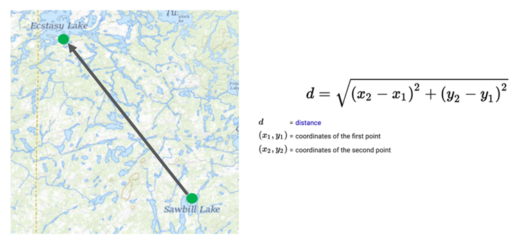
What does it mean for two concepts to be similar? Let’s start with a metaphor of a geographic map.
Given two points on the map, we can calculate a distance between these two points by using the distance formula. The inputs are just the coordinates of the two points expressed as numbers such as their longitude and latitude. The problem also can be generalized into three dimensions for two points in space. But in the three-dimensional space version, the distance calculation adds an additional term for the hight or z-axis.
Distance calculations in an embedding work in similar ways. The key is that instead of just two or three dimensions, we may have 200 or 300 dimensions. The only difference is the addition of one distance term for each new dimension.
Word Embedding Analogies
Much of the knowledge we have gained in the graph embeddings movement has come from the world of natural language processing. Data scientists have created precise distance calculations between any two words or phrases in the English language using word embeddings. They have done this by training neural networks on billions of documents and using the probability of a specific word occurring in a sentence when you take all the other words around it into account. Surrounding words become the “context window”. From this, we can effectively do distance calculations on words.
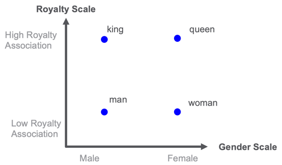
Examples of word embeddings for the concepts of royalty and gender.
In the example above, imaging putting the words king, queen, man, and woman on a two-dimensional map. One dimension is related to royalty and one dimension is related to gender. Once you have every word scored on these scales you could find similar words. For example, the word “princess” might be closest to the word “queen” in the royalty-gender space.
The challenge here is that manually scoring each word in these dimensions would take a long time. But by using machine learning and having a good error function that knows when a word can be substituted for another word or follows another word this project can be done. We can train a neural network to calculate the embedding for each word. Note that if we have a new word we have never seen before, this approach will not work.
The English language has about 40,000 words that are used in normal speech. We could put each of these words in a knowledge graph and create a pair-wise link between each word and every other word. The weight on the link would be the distance. However, that would be inefficient since by using an embedding, we could quickly recalculate the edge and the weight.
The metaphor is that just like sentences walk between words in a concept graph, we need to randomly walk through our EKG to understand how our customers, products, etc. are related.
How Are Graph Embedding Stored?
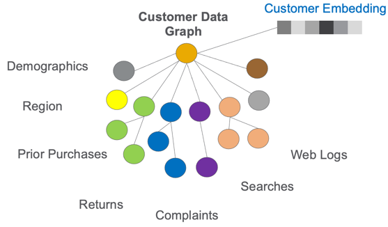
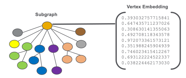
A graph embeddings are stored as a vector of numbers that are associated with a vertex or subgraph of our EKG.
An illustration of a vertex embedding for subgraph of a graph.
We don’t store strings, codes, dates, or any other types of non-numeric data in an embedding. We use numbers for fast comparison using standardize parallel computation hardware.
Size of Embeddings
Graph embeddings usually have around 100 to 300 numeric values. The individual values are usually 32-bit decimal numbers, but there are situations where you can use smaller or larger data types. The smaller the precision and the smaller the length of the vector, the faster you can compare this item with similar items.
Most comparisons don’t really need more than 300 numbers in an embedding. If the machine learning algorithms are strong, we can compress many aspects of our vertex into these values.
No Semantics with Each Value
The numbers may not represent something that we can directly tie to a single attribute or shape of the graph. We might have a feature called “customer age” but the embedding will not necessarily have a single number for the age feature. The age might be blended into one or more numbers.
Any Vertex Can Have An Embedding
Embeddings can be associated with many things in the EKG. Any important item like a customer, product, store, vendor, shipper, web session, or complaint might have its own embedding vector.
We also usually don’t associate embedding with single attributes. Single attributes don’t usually have enough information to justify the effort of creating an embedding.
There are also projects that are creating embeddings for edges and paths, but they are not nearly as common as a vertex embedding.
Calculating the Context Window of an Embedding
As we mentioned before, the area around a vertex that is used to encode an embedding is called the context window. Unfortunately, there is no simple algorithm for determining the context window. Some embeddings might only look at customer purchases from the last year to calculate an embedding. Other algorithms might look at lifetime purchases and searches that go back since the customer first visited a web site. Understanding the impact of time on an embedding, called temporal analysis, is something that might require additional rules and tuning. Clearly, a customer that purchased baby diapers on your web site 20 years ago might be very different than someone that just started purchasing them last month.
Embeddings vs. Hand-coded Feature Engineering
For those of you that are familiar with standard graph similarity algorithms such as cosine similarity calculations, we want to do a quick comparison. Cosine similarity also creates a vector of features which are also simple numeric values. The key difference is that manually creating these features takes time and the feature engineer needs to use their judgment on how to scale the values so the weights are relevant. Both age and gender might have a high weight and a feature that scores a person’s preference for chocolate or vanilla ice cream might not be relevant for general-purpose item purchases.
Embeddings try to use machine learning to automatically figure out what features are relevant for making predictions about an item.
Tradeoffs of Creating Embeddings
When we design EKGs, we work hard to not load data into RAM that does not provide value. But embeddings do take up valuable RAM. So we don’t want to go crazy and create embeddings for things that we rarely compare. We want to focus on when similarity calculations get in the way of real-time responses for our users.
Homogeneous vs. Heterogeneous Graphs
Many early research papers on graph embedding focused on simple graphs where every vertex has the same type. These are called homogeneous or monopartite graphs. One of the most common examples is the citation graph where every vertex is a research paper and all the links are to other research papers that are cited by a paper. Social networks where every vertex is a person and the only link type is “follows” or “friend-of” is another type of homogeneous graph. Word embeddings, where every word or phrase has an embedding, is another example of a homogeneous graph.
Unfortunately, knowledge graphs usually have many different types of vertices and many types of edges. These are known as multipartite graphs. And they make the process of calculating embeddings more complicated. A customer graph may have types such as Customer, Product, Purchase, Web Visit, Web Search, Product Review, Product Return, Product Complaint, Promotion Response, Coupon Use, Survey Response, etc. Creating embeddings from complex data sets can take time to set up and tune the machine learning algorithms.
How Enterprise Knowledge Graph Embeddings Are Calculated
For this article, we are going to assume you have a large EKG. By definition, an EKG does not fit in the RAM of a single server node and must be distributed over tens or hundreds of servers. This means that simple techniques like creating an adjacency matrix are out of the question. We need algorithms that scale and work on distributed graph clusters.
There are around 22,000 papers on Google Scholar that mention the topic of “graph embeddings”. I don’t claim to be an expert on all the various algorithms. In general, they fall into two categories.
Graph convolutional neural networks (GCN)
Random walks
Let’s briefly describe these two approaches before we conclude our post.
Graph Convolutional Neural Networks (GCN)
The GCN algorithms take a page from all the work that has been done with convolutional neural networks in image processing. Those algorithms look at the pixels around a given pixel to come up with the next layer in the network. Images are called “Euclidean” spaces since the distance between the pixels is uniform and predictable. GCNs use roughly the same approach by looking around a current vertex, but the conceptual distances are non-uniform and unpredictable.
Random Walk Algorithms
These algorithms tend to follow the research done in natural language processing. They work by randomly traversing all the nodes starting from a target node. The walks effectively form sentences about the target vertex and these sequences are then used the same way that NLP algorithms work.
Conclusion
I hope that the stories and metaphors in this blog post give you a better intuitive feel for what graph embeddings are and how they are used to accelerate real-time analytics. Although you might be discouraged by the fact that there is no definitive library of functions for calculating embeddings on all platforms, I think you will see from the amount of research being published that this is an active area of research. I think that just like AlexNet broke ground in image classification and BERT set a new standard for NLP, that within the next few years we will see graph embedding take center stage in the area of innovative analytics.
The importance of embeddings are a key reason why TigerGraph has developed hybrid graph+vector capability. You can store your embedding vectors in TigerGraph, link them to vertices, and perform powerful hybrid graph+vector searches.
If you want to learn more about graph embeddings and how TigerGraph can accelerate real-time analytics, contact us at info@tigergraph.abstage.xyz.
This blog post was originally featured on Towards Data Science and is written by Parker Erickson, Data Science / Machine Learning Intern at TigerGraph
Make ML Classifications Inside Your Database
Introduction
During my time at Optum, 3 trends were very important — explainable machine learning models, knowledge graph data representation, and execution of rules within those knowledge graphs. Tying these trends together, I created a method for executing decision trees inside of a TigerGraph instance.
Data Source — Banking Dataset
Data comes from a dataset hosted on Kaggle, found here. It is encouraged to read through the dataset information on the Kaggle page, but the dataset is a binary classification problem if a given customer is going to use a bank product. To train the decision tree, we only use the categorical variables in the dataset, as these can be easily modeled as vertices in our TigerGraph schema.
Input DataFrame to Decision Tree (Image by Author)
Decision Tree
A decision tree is a machine learning model in which nodes are organized in a tree structure, where each node is a conditional statement, such as checking if an attribute of a datapoint is present. These trees are trained to use a minimum number of conditions in order to classify a datapoint. Decision trees are easy to interpret, as each node has a clear meaning to what feature it is testing for in its conditional expression. This explainability of a decision tree’s classification separates it from other machine learning model types such as deep neural networks.
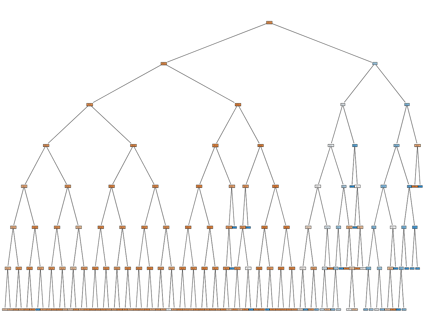
To train the decision tree, we use sklearn in a Python Jupyter Notebook, using only the aforementioned categorical variables. Using a maximum depth of 7, we achieve an accuracy of 89% (note that the dataset is imbalanced, so this isn’t the best metric, but serves our purposes for now). Here is the outputted tree:
Trained Decision Tree (Image by Author)
Once the decision tree was trained, a Pandas dataframe was constructed that consisted of the edges between each node in the decision tree, to eventually be upserted into our TigerGraph instance.
TigerGraph
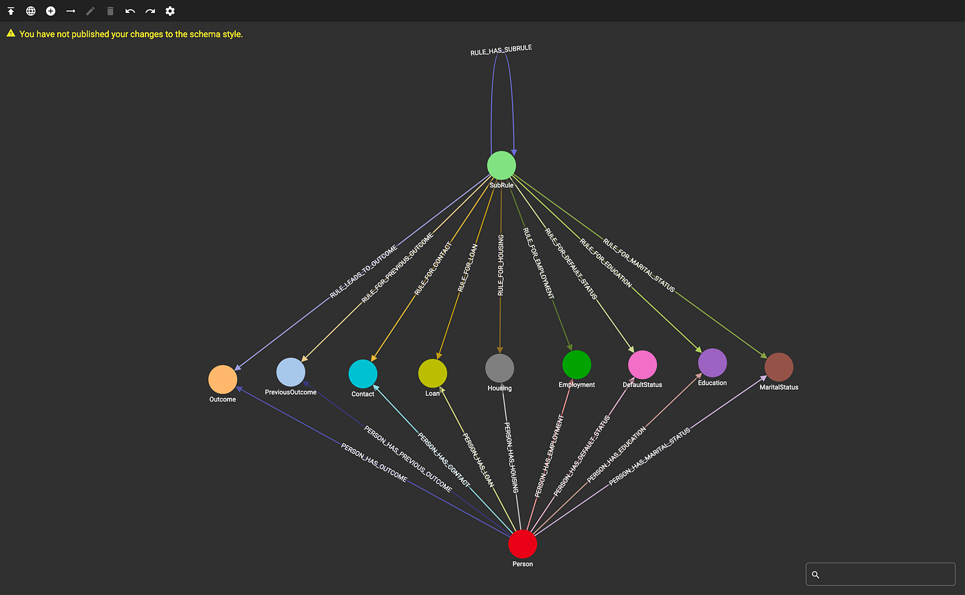
The data was modeled in TigerGraph such that each outcome (signing up or declining the bank product), along with each individual and categorical attributes were a vertex type. Additionally, a “SubRule” vertex is introduced, which models each node in the decision tree. Each of these vertex types were connected to one another by a series of edges defined by the schema, pictured below:
TigerGraph Schema (Image by Author)
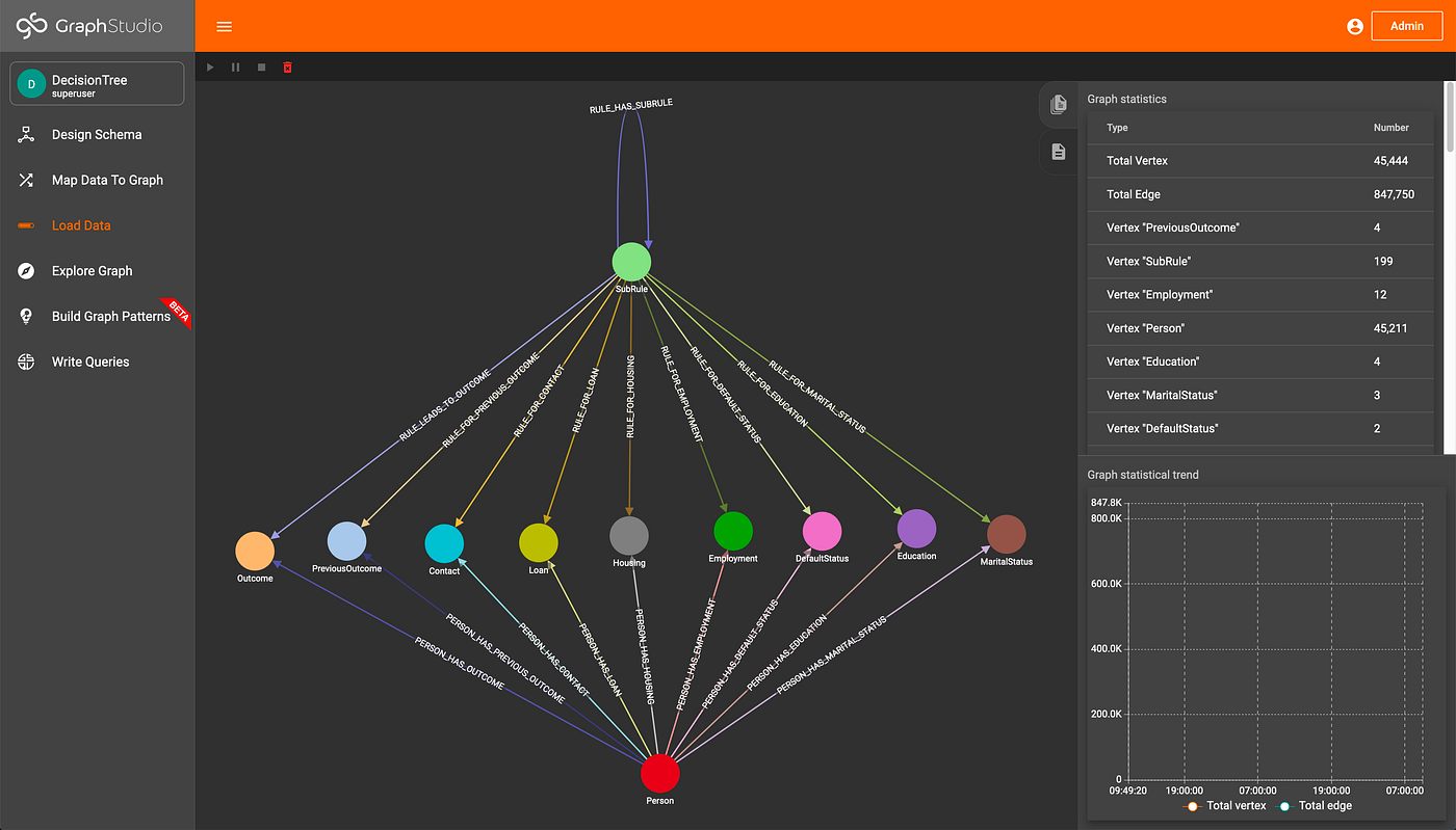
Two loading scripts are defined to load the data and decision tree into the TigerGraph instance, written with pyTigerGraph. Once these scripts are run, we can see how much data is in the graph:
Data Loaded (Image by Author)
Accumulators in TigerGraph
According to the TigerGraph documentation, “Accumulators are special types of variables that accumulate information about the graph during its traversal and exploration.” The accumulators can be either global or local, where local accumulators are bound to each individual vertex, and global accumulators are graph-wide. This element of GSQL allows code to be very compact and easily understood. For more, check out the TigerGraph documentation.
Traversal Query
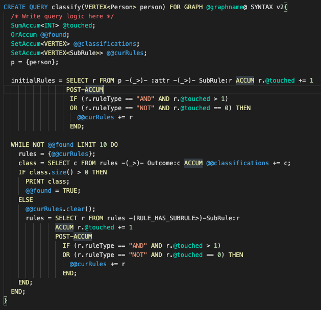
The query that traverses the decision tree and makes classifications utilizes multiple accumulators. To start, given an individual in the graph, we gather all of their attributes by traversing the graph. From these attributes, we can see what SubRules apply to those attributes by simply traversing from the attributes to the SubRules. Each SubRule is then assigned a running count as to if it has been traversed to before. Since decision trees operate on AND as well as NOT operations, the SubRules are then iteratively filtered down to valid rules by checking the number of times they have been touched, until a classification has been reached.
Classification Query (Image by Author)
The classify query is very simple and compact (about 30 lines of code) due to the power of accumulators and the graph structure, especially when compared to other rules engines with about 10k lines of code. Since the rules are defined in the graph and classifications are made by traversing edges within the graph, the performance is much higher than traditional rule engines such as one based on SQL and Drools since TigerGraph can typically traverse about 2 million edges per second per thread of execution.
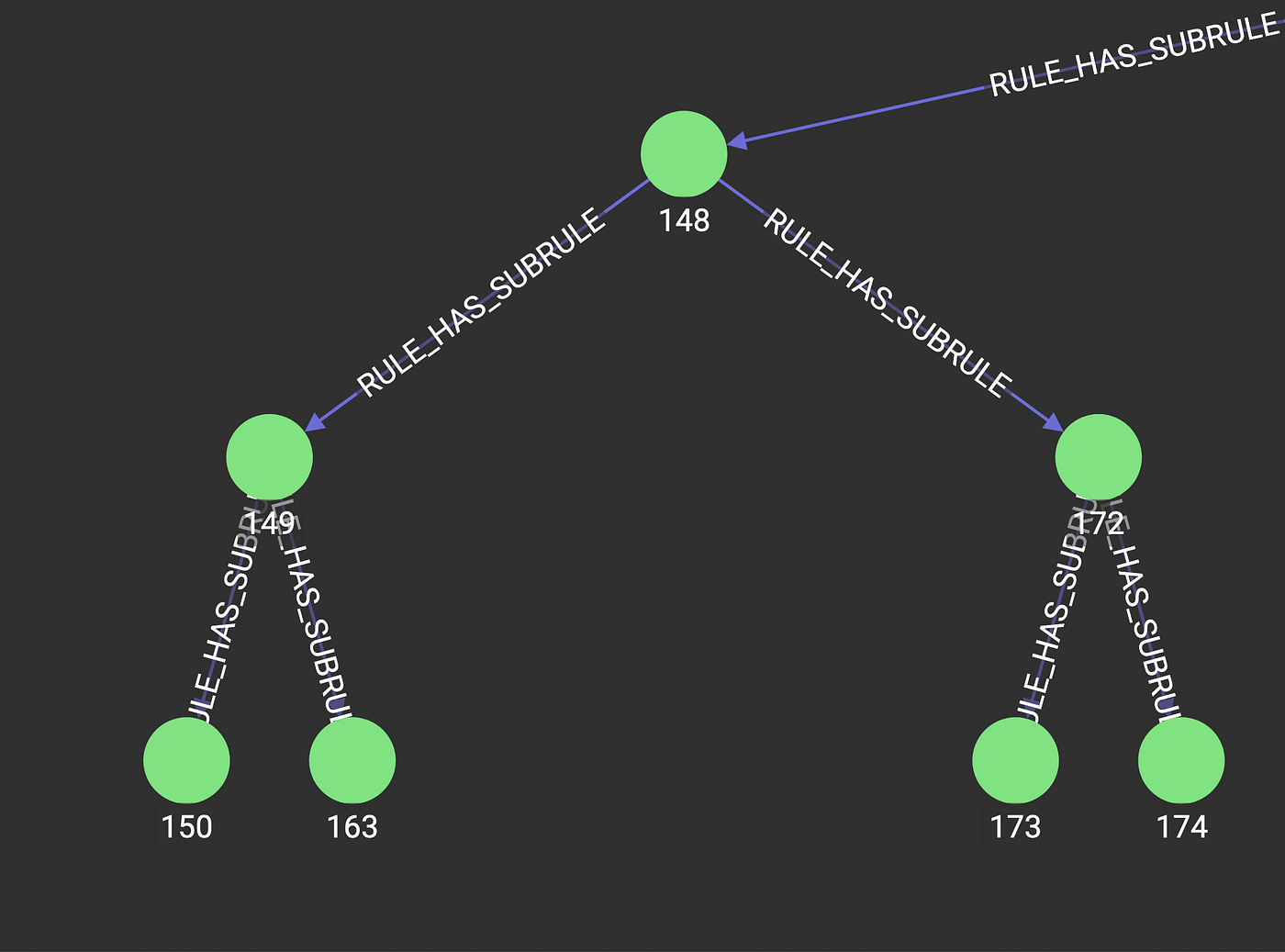
Additionally, we can explore the decision tree inside of TigerGraph GraphStudio, the GUI visualization tool, in order to help understand why a classification was made for an individual.
Excerpt of Decision Tree in TigerGraph (Image by Author)
Conclusion
This setup will allow users to run interpretable machine learning models inside of TigerGraph, where their data resides. Many different business processes, such as claims adjudication, can be represented as decision trees, and could be executed within the knowledge graph. Additional further work could be done to train the decision tree model within TigerGraph, removing the need to move the data in and out of the instance. All code can be found here: https://github.com/parkererickson/tigergraphDecisionTree.