Optimized Counting of Common Neighbors/Vertices in GSQL
Graph analytics plays a crucial role in finding hidden relationships within large datasets. One fundamental operation in this domain is calculating the number of common neighbors between pairs of vertices in a graph. This has applications in similarity measurement, link prediction, graph compression, community detection, and more.
Current multi-threaded approaches often rely on set intersection techniques or do not easily lend themselves to parallelization. In this blog post, we’ll explore:
- An optimized algorithm for counting common neighbors that outperforms the set intersection method.
- How to implement this optimized algorithm in GSQL, a Turing-complete language.
- A comparative performance analysis of both methods.
1.0 Counting Common Neighbors/Vertices
In a graph, vertices (also known as nodes) represent entities, and edges signify relationships between those entities. If an edge connects two vertices, we say those vertices are neighbors. If vertex C is a neighbor of vertex A, and C is also a neighbor of vertex B, we say that C is a common neighbor of A and B.
Some use cases that can utilize the common neighbors are described below:
- Community Detection: Identifying vertices that have a high number of common neighbors can indicate that they belong to the same community or cluster within the graph.
- Recommendation Systems: Common neighbors can be used to make recommendations. If two users in a social network have common friends, it might suggest they have shared interests.
- Link Prediction: Analyzing common neighbors can help predict potential connections between vertices that are not directly linked yet. If two vertices share many common neighbors, there’s a higher chance they might form a direct connection in the future.
- Graph Similarity: Comparing the sets of common neighbors between vertices can be used to measure the similarity or relatedness of vertices within the graph.

1.1 Merchant-Merchant Graph Use Case
In the use case below, we will be using a graph that captures how strongly two Merchants, represented by point-of-sale (POS) devices, are connected to each other based on common distinct credit or debit Cards that are used at both Merchants. See Figure 1 below.
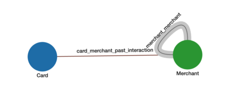 Figure 1. Merchant-to-merchant graph schema.
For the Merchant-Merchant Graph:
- Each Merchant vertex and Card vertex represents a distinct entity
- The edges card_merchant_past_interaction come directly from Card (shopper) to Merchant transactions.
- The weighted edges merchant_merchant between two Merchants represents how many common Cards are shopping between the two Merchants. These edges and their weights are not in the original data but are the result of analyzing the graph. The higher number of common Cards between two Merchants, the higher the weight and stronger the connection.
If a shopper is shopping at a given Merchant, we can use the strengths of connections to predict which other merchants they are most likely to shop at (recommendation). Or this metric can also be used as a signal for fraudulent transactions (fraud detection).
The schema for our graph looks like below where card_merchant_past_interaction edges are already available to us and we want to insert merchant_merchant edges and their corresponding weight.
Figure 2 shows an example of how merchant_merchant weighted edges would be inserted. The edge weight inserted between the two Merchants is 4 because 4 cards are in common between the two Merchants:
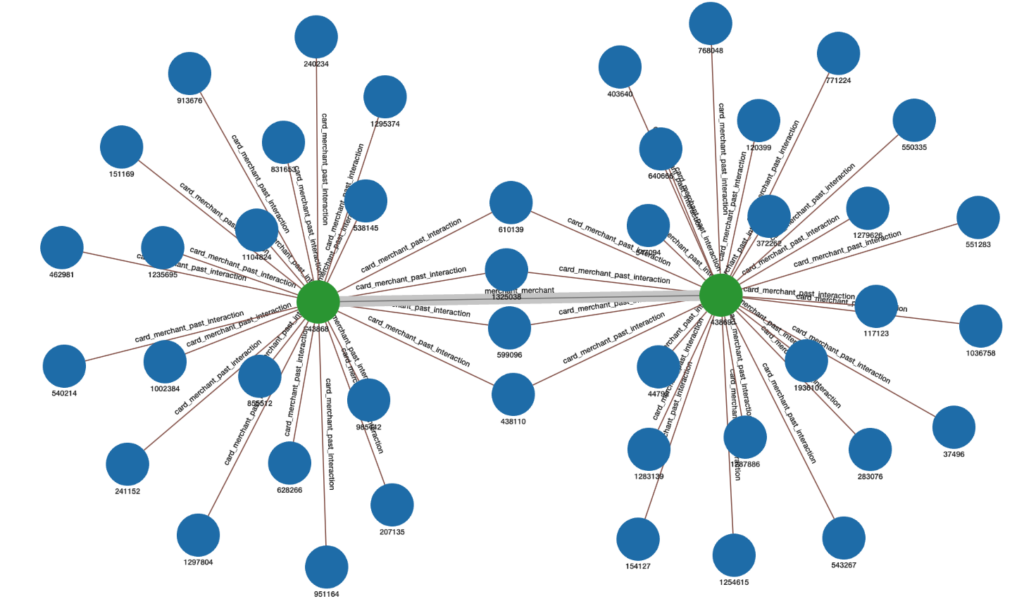
Figure 2. Example of weighted edge representing the number of common Cards between two Merchants.
2.0 Complexity Analysis and Optimization
2.1 Time Complexity of the Naive Intersection Method
To count the common neighbors (Cards in this case) between two given (Merchant) vertices A and B, we can collect the set of Card neighbors of A, those of B, and do a set intersection between the two. The time complexity for this algorithm can be determined as follows:
- Getting Neighbors for Vertex A and B: Retrieving the set of neighbors for a single vertex in an adjacency list representation of an undirected graph takes O(K) time, where K is the degree (number of incident edges) of the vertex. So, for vertices A and B it would take O(K_a + K_b) time to collect the sets of neighbors.
- Calculating Intersection: Finding the intersection of two sets with sizes n and m would generally require O(n+m) time. In our case, n=K_a and m=K_b, the number of neighbors for vertices A and B, respectively.
Time complexity for a single pair:
Combining these steps, the time complexity to calculate the Common Neighbors for a single pair of vertices (A,B) would be O(K_a + K_b).
Time complexity for all pairs:
For calculating Common Neighbors for all possible pairs of n vertices in the graph, we would need to perform this calculation n(n-1)/2 times, leading to a worst-case time complexity of O(n2K), where K is the maximum degree in the graph.
It is possible to not count intersections for all n2 pairs. To be a common neighbor, a (Card) vertex must have at least two neighbors. For each card, we can collect its list of neighboring Merchants and only continue to work with those having degree K ≥ 2. This takes O(nK) time. We only need to calculate the intersection between Merchants on these neighbor lists. The worst case length of this list would be degree K. Hence the new worst case time complexity for n vertices becomes O(nK2).
2.2 Optimized Time complexity
The optimized method aims to reduce the time complexity by altering the approach to how we count the common neighbors (or “Cards”) between two vertices (or “Merchants”) A and B. Instead of creating sets of neighbors for two merchants A and B and then finding their intersection, this method uses a direct counting approach.
Consider the Example of three Cards (C1,C2,C3) and five Merchants (M1,M2,M3,M4,M5) connected as in Figure 3:
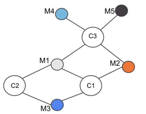
Figure 3. Merchant-Card graph example
Our objective is to find the number of common cards between each Merchant-Merchant pair.
Consider Merchant pair (M1,M3). To compute the common Cards between M1 and M3, find the set of Cards neighboring M1, i.e., S1 = {C1,C2,C3}. Next find the set of Cards neighboring M3: S2 = {C1,C2}. Now if we run the intersection , we see the set size is 2, i.e., 2 cards are common between M1 and M3. Running for all Merchant pairs M1 to M5, we can get the edge weight for all pairs of Merchants with O(nK2) complexity.
However, instead of doing intersection for each merchant pair, we can compute the edge weight using the following steps:
- Find the set of all Merchants shopped at by a Card (neighbors of the Card)
- For each Card, get each pair of Merchants in the set and do:
- Add a merchant_merchant edge if it doesn’t exist, with initial weight of 0
- Increment edge weight by 1
So for our example above in Step 1, we find all neighbors of each Card:
- C1 Set: (M1,M2,M3)
- C2 Set: (M1,M3)
- C3 Set: (M1,M2,M4,M5)
And then we iterate over each card and each Merchant pair in the set, incrementing the edge weight by 1:
- For C1 edge weight update applied:
- (M1,M2) += 1 → 1
- (M2,M3) += 1 → 1
- (M1,M3) += 1 → 1
- For C2 edge weight update applied:
- (M1,M3) += 1 → 2
- For C3 edge weights update applied:
- (M1,M2) += 1 → 2
- (M1,M4) += 1 → 1
- (M1,M5) += 1 → 1
- (M2,M4) += 1 → 1
- (M2,M5) += 1 → 1
- (M4,M5) += 1 → 1
Hence the final edge_weight pairs are as shown in Figure 4:
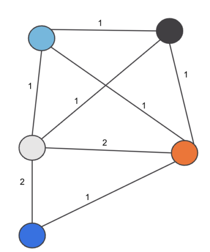
Figure 4. Weighted edges between Merchants
Hence we see from the example the time complexity can be optimized by observing the fact that we can count the number of common vertices between two vertices instead of doing an intersection and the counting operation can be done in O(1) and hence the complexity can be reduced from O(n K2) to O(nK).
3.0 Implementation in TigerGraph Using GSQL
To execute Common Neighbors algorithms, we will utilize the TigerGraph database as our graph data storage and use GSQL for algorithm implementation. Because of TigerGraph’s distributed nature we can run the algorithm distributedly and with memory efficiency.
We will evaluate performance differences between the intersect method and the optimized approach by using the above pre-established use-case: calculating common cardholders who shop at two different merchants and then assigning a weighted edge between those merchants based on that count.
The files for building Schema/Load Data and running queries in TigerGraph are in the appendix.
3.1 Intersect method GSQL implementation:
The query below shows the implementation of the Intersection method and how to insert the merchant-merchant edges in O(nK2) time.
CREATE DISTRIBUTED QUERY _02_common_cards_intersect(
  INT min_edge_weight = 1
)
FOR GRAPH optimizing_common_neighbors {
  SetAccum @merchants;
  MapAccum<VERTEX, INT> @edge_weight;
  DATETIME before;
  cards = {Card.*};
  before=(now());
  // Collect all Merchants on the Card
  merchants = SELECT m FROM cards:c- (card_merchant_past_interaction:e) - Merchant:m
              ACCUM c.@merchants+=m; //O(M) where M= number of cards
  PRINT "Time to collection of merchants on cards ",datetime_diff(now(), before);
  // INSERT edges and weights using the INTERSECT method.
  before=(now());
  temp = SELECT m FROM merchants:m -(card_merchant_past_interaction:e)- Card:c
          ACCUM
            FOREACH merc IN c.@merchants DO // O(N*K) where N =number of Merchants and K= Max degree of Card
              IF getvid(m) < getvid(merc) THEN
                tg_common_neighbors(m,merc,min_edge_weight) //O(K_a+K_b) where K_a and K_b are the degrees of the merchant pair
              END
            END; //Total complexity O(N*K*(K_a+K_b))=O(N.K^2)
  PRINT "Time to INSERT edges using intersect method",datetime_diff(now(), before);
}
The sub-query tg_common_neighbors called in the above query does the actual intersection in O(K_a + K_b) time.
Below is the sub query logic:
//Intersect subquery
CREATE QUERY tg_common_neighbors(
  VERTEX v_source,
  VERTEX v_target,
  INT min_edge_weight
)
FOR GRAPH optimizing_common_neighbors {
  avs = {v_source};
  bvs = {v_target};
  INT sz;
  na = SELECT n
       FROM avs -(card_merchant_past_interaction:e)- :n;
  nb = SELECT n
       FROM bvs -(card_merchant_past_interaction:e)- :n;
  # Get neighbors in common for source and target and compute the common neighbors
  u = na INTERSECT nb;
  sz=u.size();
  # Insert edge only if the weight is >= min_edge_weight
  IF sz >= min_edge_weight THEN
    INSERT INTO merchant_merchant (FROM ,TO ,weight) VALUES (v_source,v_target,sz) ;
  END;
}
3.2 Optimized Common Neighbors implementation
For optimization we simply replace the intersect sub query tg_common_neighbors by counting the edge weight for each merchant-merchant vertex pair and hence reduce the complexity to O(K).
CREATE DISTRIBUTED QUERY _02_common_cards_optimized(
  INT min_edge_weight = 1
)
FOR GRAPH optimizing_common_neighbors {
  SetAccum @merchants;
  MapAccum<VERTEX, INT> @edge_weight;
  DATETIME before;
  cards = {Card.*};
  before=(now());
  // Collect all Merchants on the Card
  merchants = SELECT m FROM cards:c- (card_merchant_past_interaction:e) - Merchant:m
              ACCUM c.@merchants+=m; //O(M) where M= number of cards
  PRINT "Time to collection of merchants on cards ",datetime_diff(now(), before);
  // Establish logical edges an summed weights
  before=(now());
  temp = SELECT m FROM merchants:m -(card_merchant_past_interaction:e)- Card:c
          ACCUM
            FOREACH merc IN c.@merchants DO // O(N*K) where N =number of Merchants and K= Max degree of Card
              IF getvid(m) < getvid(merc) THEN m.@edge_weight += (merc -> 1) //O(1)
              END
            END; //Total complexity O(N*K*1)=O(N.K)
  PRINT "Time to establish merchant-merchant edges using optimized common neighbors ",datetime_diff(now(), before);
  // Insert edges
  before=(now());
  temp = SELECT m FROM merchants:m
          POST-ACCUM
            FOREACH (merc, w) IN m.@edge_weight DO
              IF w >= min_edge_weight THEN                 // Insert edge only if the weight is >= min_edge_weight
                  INSERT INTO merchant_merchant VALUES (m, merc, w)
              END
            END;
  PRINT "Time to INSERT merchant-merchant edges  ",datetime_diff(now(), before);
}
4. Performance Comparison
For comparing the performance of the two algorithms the data metrics and hardware being used are as follows:
Data Metrics:
| Metric | Count |
| All Vertices | 1,807,672 |
| All Edges | 6,872,163 |
| Vertex “Card” | 1,335,486 |
| Vertex “Merchant” | 472,186 |
| Edge “card_merchant_past_interaction” | 6,872,163 |
| Edge “merchant_merchant” | 0 |
Raw Data size = 95.1MB.
The final count of “merchant_merchant” edges inserted is 20,607,316.
Hardware Configuration:
2 x TG.C16.M64 TigerGraph Cloud instances (16 CPUs, 64GB Memory)
The following Table captures the performance of the two algorithms.
| Metric | Intersection Method | Optimized Method | Notes |
| Execution Time (Seconds) | 3517.49 | 23.33 | 153x Speed improvement |
| Peak Memory Usage (GB) | 8.1 | 2.1 | 4x Memory reduction |
Lorem ipsum dolor sit amet, consectetur adipiscing elit. Ut elit tellus, luctus nec ullamcorper mattis, pulvinar dapibus leo.
5.0 Conclusion
The optimized algorithm significantly outperforms the intersection-based approach, not just in speed but also in memory efficiency. TigerGraph’s GSQL enables users to tailor algorithms to their specific needs, offering unparalleled flexibility and scalability. For additional examples of graph algorithms implemented in GSQL, please refer to our Graph Data Science Library.
Appendix
Solution that can be run in GSQL shell
Notebook to create Schema/Load_data/install queries
Graph Data File for Card-Merchant Edges
If you’re interested in exploring how TigerGraph can open up new dimensions with your data, you can sign up for a free instance of TigerGraph Cloud at tgcloud.io or contact us at info@tigergraph.abstage.xyz.
Introduction
Hello everyone! I’m Xuanlei Lin. I have worked as a solution engineer at TigerGraph for two years and as a customer success consultant for another two years. Throughout this period, I have been involved in over 60 projects utilizing TigerGraph. In this blog, I would like to introduce you to a powerful feature of TigerGraph called multi-edge. Multi-edge refers to a concept in graph theory where multiple edges, or connections, exist between two nodes in a graph. In a traditional graph, each pair of nodes can have at most one edge connecting them. However, in a multi-edge graph, two nodes can be connected by multiple edges, indicating different types of relationships or interactions between them. Multi-edge graphs are often used to model complex systems where multiple interactions or relationships exist between entities.
Recently, I had the opportunity to leverage the multi-edge functionality to assist an insurance customer in implementing temporal search for agent hierarchy. While this project was specific to the insurance industry, multi-edge is a solution for temporal search for many other industries and use cases.
In this blog post, I will present a simplified version of the demo based on the project I recently completed. Firstly, I will outline the business requirements and the technical challenges associated with their implementation. Next, I will introduce a solution that leverages TigerGraph’s multi-edge functionality. Additionally, I will explore further use cases of multi-edge in the insurance industry and other sectors.
Requirements
Before we begin, let me provide some background information on the business domain. In the insurance industry, particularly in life insurance companies, agents, also referred to as salespersons, play a crucial role as the primary sales channel for insurance policies. A large insurance company may have many thousands of agents organized into multi-level groups. The hierarchical structure consists of groups at the lowest level, departments in the middle, and regions at the highest level. Each group/department/region is overseen by a manager, and every agent belongs to one specific group/department/region.
Apart from the hierarchical relationships, there are two additional types of relationships between agents. The first is the introduction relationship, where any agent can recommend new agents to the company. The second is the fostering relationship, which occurs when an agent is promoted to a higher managerial position within a group/department/region. In this case, the agent’s former direct leader establishes a fostering relationship with the agent. The fostering relationship can be further categorized into three types based on the level of the new rank attained by the fostered agent: group, department, and region.
Let’s consider the leftmost group in Figure 1 as an example. Agents D, F, H, and K form a group, with D serving as the group manager. D is the manager of F, H, and K. D introduced F and H, and H introduced K. Agent B has a group fostering relationship with D.
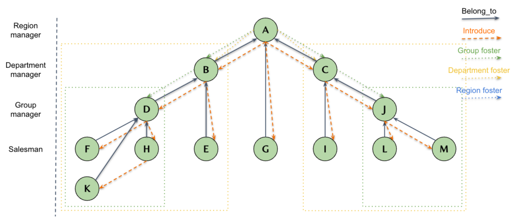
Figure 1
The hierarchy, introduction, and fostering relationships play a vital role in the performance appraisal of agents. The commission structure for agents consists of both direct and indirect commissions. The direct commission refers to the commission earned from the insurance policies sold by the agent personally. On the other hand, the indirect commission refers to the commission earned from the policies sold by other agents.
To illustrate, let’s consider an example: Agent A sells an insurance policy and receives a direct commission for the sale. However, not only does Agent A receive a commission, but A’s manager, introducer, and the agent who fostered Also receive a portion of the commission. This means that when Agent A sells a policy, their manager, the agent who introduced them, and the agent who fostered A all receive a share of the commission.
Challenges
As mentioned earlier, there are various relationships between agents, and the complexity arises from the fact that these relationships are subject to change over time. The company promotes or demotes agents on a monthly basis, based on their performance. Additionally, new agents join the organization while old agents may leave. Essentially, this creates a temporal graph where relationships evolve over time.
Traditional technologies like relational databases or big data solutions often struggle to effectively manage and maintain these dynamic relationships. Prior to joining TigerGraph, I was involved in a similar project where extensive SQL and Java code were required to implement the functionality. Unfortunately, the resulting codebase became incredibly complex, making it difficult for anyone to fully comprehend and maintain.
Solution
The challenges posed by this project may indeed be daunting for traditional technologies, but they are well within the capabilities of TigerGraph. Firstly, the scale of millions of agents is not a significant concern for TigerGraph, as it can support billions or even trillions of vertices. Secondly, TigerGraph excels in handling complex relationships and can effectively represent intricate connections.
The only difficulty lies in managing temporal relationships. Customers require the ability to view the latest agent hierarchy while also being able to trace the agent hierarchy back to a specific point in time. In earlier versions of TigerGraph, multi-edge support was lacking. As a workaround, an additional vertex type was introduced to record historical data between vertices. However, this workaround is no longer necessary due to the introduction of multi-edge, a more elegant and high-performance solution. Multi-edge allows for the existence of multiple edges of the same type between a pair of vertices. To differentiate between different edges between a pair of vertices, a Discriminator has been added, which can be understood as a primary key on the edge. For example, the following code is used to create edges representing the management relationship.
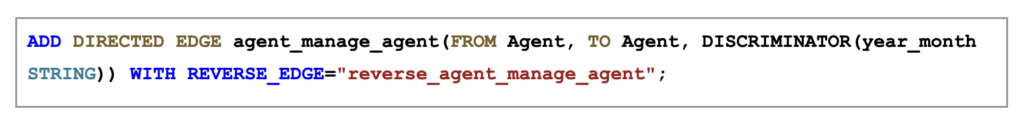
The schema design consists of a single vertex type, “Agent,” and an edge type, “agent_manage_agent,” which incorporates the “year_month” Discriminator to differentiate the management relationships for each month.
Below is the complete schema design:
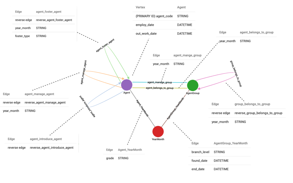
After designing the schema and loading the data, we can create a query to perform the temporal search. This query will enable us to search for the hierarchy of agents at a specific moment in history. For example, if we input the date “2008-01-01,” the resulting agent hierarchy at that particular time would be as follows:
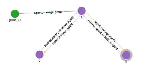
Figure 2
Next, if we input the date “2014-01-01,” we will obtain the following results:
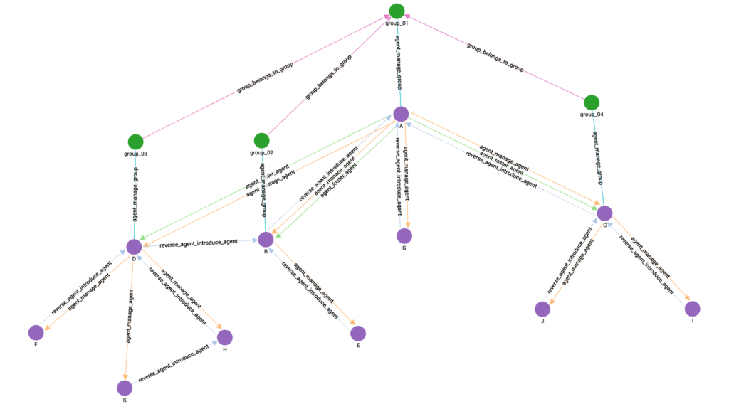
Figure 3
Lastly, if we input the date “2019-01-01,” we will obtain the following results:
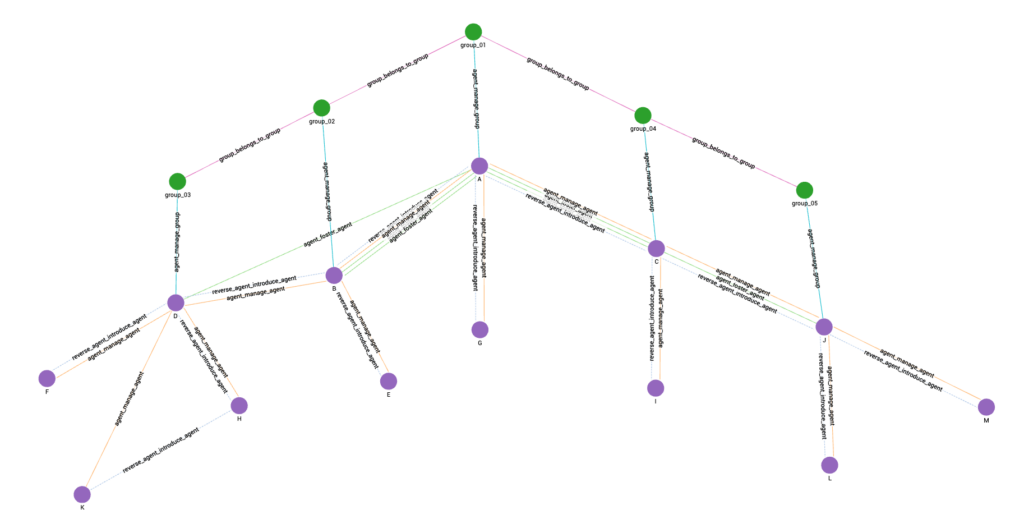
Figure 4
It should be noted that the agent hierarchy depicted in Figure 4 is the same as the one shown in Figure 1.
Further applications
As mentioned earlier, the above demo is just a simplified version. In actual projects, after establishing the temporal graph for the agent hierarchy, we can also associate more entities such as policies, applicants, insured individuals, claims, and commissions.
Once a more complete schema is established, we can have more diverse applications. For example:
- Based on the latest agent hierarchy, precalculate the performance of all agents for the upcoming months, end of quarters, and year-end, and make adjustments to the agent hierarchy based on performance precalculation.
- Look back at the historical agent hierarchy, and perform data analysis based on the agent hierarchy at that time.
- Combine with machine learning, extract features, and conduct retrospective testing.
The application of multi-edge in other industries
Multi-edge is a versatile technology that can be applied in various industries. In the telecommunications industry, there can be multiple connections between phones. In the banking industry, there can be multiple transactions between accounts. In the manufacturing industry, each component can have multiple parameters, and each parameter may have been measured at different times. All of these can be addressed using multi-edge.
Many more examples can be given, and you can apply the concept of multi-edge based on the characteristics of your industry’s data. I believe that using multi-edge can help you store data more effectively, write queries more conveniently, and retrieve information faster.
If you’re interested in exploring how TigerGraph can open up new dimensions with your data, you can sign up for a free instance of TigerGraph Cloud at tgcloud.io or contact us at info@tigergraph.abstage.xyz.
First in our series of blogs straight from our engineers to you.
In today’s digitally interconnected world the proliferation of data has presented both unprecedented opportunities and challenges. One of these challenges is the need to accurately identify and link entities across various datasets, a process known as entity resolution. Enter TigerGraph – a native parallel graph database and analytics platform revolutionizing the field of entity resolution. This blog post explores the benefits of utilizing TigerGraph for entity resolution, both in batch and real-time scenarios, and highlights its role in fortifying fraud detection mechanisms, particularly in combating identity fraud.
TigerGraph’s unique architecture based on graph database technology offers several advantages that make an ideal choice for handling entity resolution tasks:
- Flexible Data Model: TigerGraph’s native graph model allows for intuitive representation of complex relationships and hierarchies between entities. This flexibility is crucial for accurately identifying and linking entities across disparate data sources.
- Efficient Parallel Processing: TigerGraph’s native parallel processing capabilities enable rapid data ingestion, processing, and querying. This is crucial for both batch processing and real-time scenarios where quick decision-making is paramount.
- Scalability: TigerGraph’s distributed nature ensures seamless scalability as data volumes grow. This scalability is essential for accommodating ever-expanding datasets and maintaining high-resolution accuracy.
- Advanced Algorithms: TigerGraph provides a rich library of graph algorithms that can be seamlessly integrated into entity resolution workflows. These algorithms help uncover hidden connections and similarities between entities, enhancing the accuracy of the resolution process.

Benefits of TigerGraph for Entity Resolution
- Accurate Linkage: TigerGraph’s ability to capture intricate relationships between entities leads to more accurate linkage, reducing false positives and negatives in the entity resolution process.
- Real-time Insights: In scenarios where real-time identification is critical, TigerGraph’s low-latency query performance ensures timely insights, enabling proactive fraud detection and prevention.
- Holistic View: TigerGraph’s graph-based approach allows for a holistic view of entities by capturing not just direct relationships but also indirect associations. This helps in identifying complex patterns of fraud that might be missed using traditional methods.
TigerGraph and Identity Fraud Prevention
Identity fraud is a pervasive and rapidly evolving form of fraud that can have far-reaching consequences for individuals and organizations. TigerGraph plays a pivotal role in safeguarding against identity fraud through its entity resolution capabilities:
- Pattern Detection: TigerGraph’s graph algorithms can identify suspicious patterns that indicate potential identity fraud, such as multiple accounts linked to a single entity or unusual cross-network interactions.
- Behavior Analysis: By tracking and analyzing the behavior of entities over time, TigerGraph can detect anomalies and deviations from established patterns, flagging potential identity fraud attempts
- Watchlist Matching: TigerGraph can efficiently match entities against watchlists and historical data to identify known fraudulent actors, helping prevent their unauthorized access or transactions.
- Collaborative Intelligence: TigerGraph can facilitate collaboration between different departments or organizations by providing a unified platform for sharing and analyzing entity data. This enhances the collective ability to combat identity fraud on a larger scale.
Example
The following is an example based on a real use.
Schema
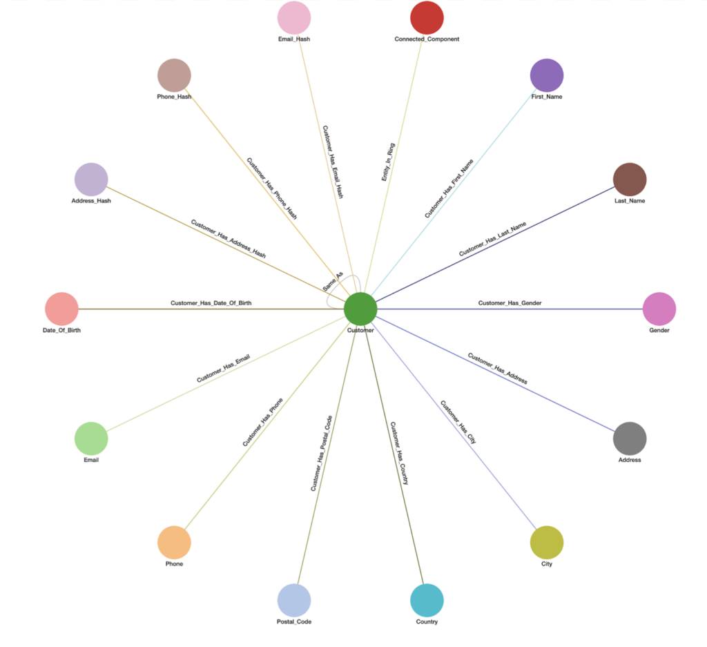
In the below schema Entity Resolution is being performed on the Customer entity using 10 PII attributes (First_Name, Last_Name, Gender, Address, City, Country, Postal_Code, Phone, Email, and Date_of_Birth). The 3 _Hash vertices are used to store minHash values for respective Address, Phone, and Email fuzzy matching. All queries support weighted PII attribute(s) and threshold that can be statically or dynamically set per request. The entity can be any data vertex and PII attribute(s) can be any 1-hop neighbor vertex(ices) from the entity.
Matching Methods
The solution matches entities based on several criteria. Each criterion translates to its own relational pattern in the graph.
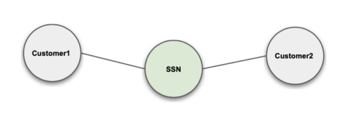
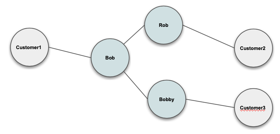
Exact Match
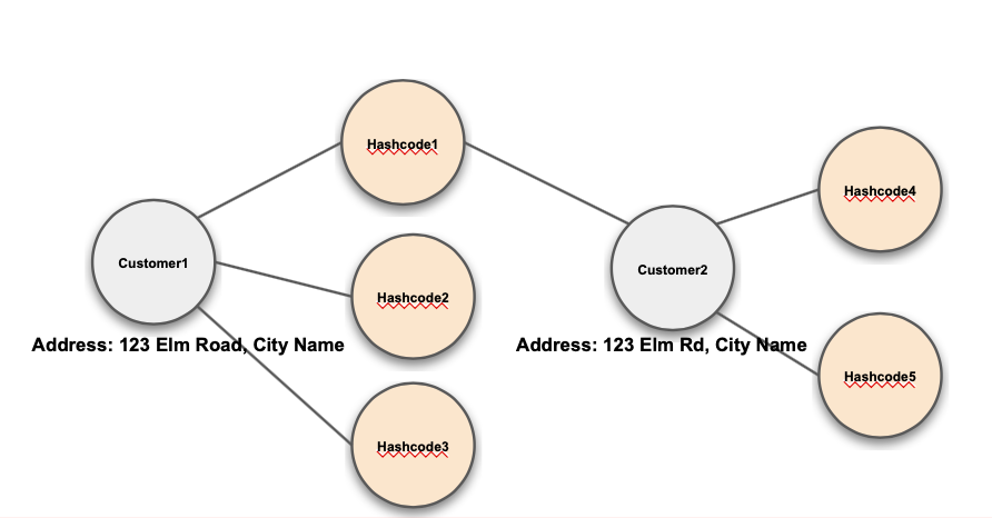
MinHash Fuzzy Match: connects entities using minHash
Metaphone / Soundex Match
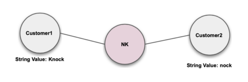
Nickname
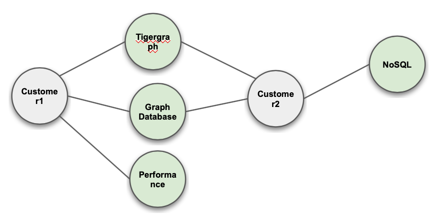
Keyword Extraction
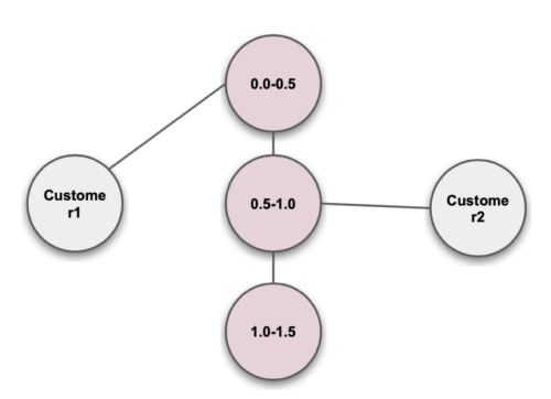
Continuous Value
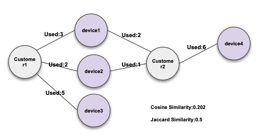
Cosine / Jaccard Similarity
Geo-Location
GSQL Queries & Endpoints
The solution is then implemented as a series of GSQL graph queries.
- delete_all_connected_componentsFirst query executed as part of the full graph Entity Resolution process to remove all existing Connected_Component relationships so these can be fully reset.
- match_entitiesBatch Weakly Connected Components (WCC) algorithm query executed as part of the full graph Entity Resolution process to match all entities using the predetermined matching logic with dynamic weighting per attribute and threshold parameters. After this query completes any matching entities will be connected with a “Same_As” edge in the graph.
- unify_entitiesThird and final query executed as part of the full graph Entity Resolution process to assign all entities in the graph into a Connected_Component vertex. After this query completes all entities connected with a Same_As edge from the previous matching step will be assigned to a common Connected_Component community in the graph and any entities unable to be matched will be assigned to their own distinct Connected_Component community.
- incremental_er (Real-Time ER)Approximate Weakly Connected Components (WCC) algorithm query executed as part of real time Entity Resolution process accepting JSON payload of all entity and PII vertex values which is upserted to the graph and returns boolean entity_resolution status indicating if incoming payload matches with any existing entities in near real time. If matching happens the new entity will be added to the respective Connected_Component after this query completes. If matching does not happen the new entity will be added to a Connected_Component following the next full graph Entity Resolution process.
- distance_and_path_to_XXX
where XXX is other entity(ies) with attribute such as “fraud_status == True”Optional query executed as part of real time Entity Resolution and following incremental_er accepting entity vertex (expected to use the same entity as previous incremental_er query) as input and returns graph features including distance and path to nearest entity(ies) up to configurable amount of maximum hops away with a particular attribute such as fraud_status is True.</>
- get_cc_statsOptional query executed as part of real time Entity Resolution and following incremental_er accepting entity vertex (expected to use the same entity as previous incremental_er query) as input and returns graph features on the associated Connected_Component such as number of unique entities, each node, how many entities are connected by PII attributes, etc.
Integration Interaction Pattern
The full graph Entity Resolution process (delete_all_connected_components, match_entities, and unify_entities) is generally run at least daily but can be run more often such as hourly or every X hours per day. The real time Entity Resolution process (incremental_er, distance_and_path_to_, and get_cc_stats is event driven to enhance real time decision making models with graph features for financial application approvals/denials or other entities/labels etc.
Conclusion
In the dynamic arena of Anti-Money Laundering (AML), the conventional rule-based approach to spotting potential financial crimes is yielding to the transformative potential of graph machine learning. The escalating volume of financial transactions and the prevalence of false positive alerts have catalyzed the adoption of innovative techniques that prioritize investigation efficiency. Graph machine learning, with its ability to decipher intricate relationships between entities in financial data, emerges as a pivotal solution. By leveraging graph features and advanced Graph Neural Networks, institutions can not only mitigate false positives but also enhance investigative accuracy. In this landscape, TigerGraph’s prowess shines – its scalability and performance in generating graph features have positioned it as a leader. As financial institutions navigate the complex terrain of AML, the convergence of graph machine learning and TigerGraph’s capabilities promises a more resilient defense against money laundering while optimizing resource allocation for investigations.
Download TigerGraph’s O’Reilly book Graph-Powered Analytics and Machine Learning. This book uses use case examples, including entity resolution and financial crime detection, to teach about graph analytics and graph machine learning. The examples in the book can be tried for free on TigerGraph Cloud.