The Five Graph Algorithms Every Data Leader Needs to Know
Most data leaders are fluent in metrics. They understand revenue trends, customer acquisition costs, churn rates, and performance dashboards. They can interpret forecasts, run regression models, and evaluate model accuracy.
That fluency matters, but modern enterprise systems are no longer defined by isolated metrics. They are defined by connections.
Key Takeaways
- Modern enterprise systems are defined by connections, not isolated metrics.
- Graph algorithms measure structural influence, coordination, and propagation inside connected networks.
- Centrality identifies structurally important entities.
- Community detection reveals hidden clusters and coordinated groups.
- Pathfinding exposes how risk or influence travels.
- Similarity compares entities based on shared relationships rather than attributes.
- Ranking prioritizes action by surfacing the most structurally significant nodes.
- These algorithms move analytics from descriptive reporting to structural reasoning.
Supplier disruptions do not stay isolated; they move through dependency chains. Customer communities shape demand in ways that raw counts cannot explain. Interconnected accounts can distort risk signals across an entire portfolio. Even a single logistics bottleneck can propagate across regions.
In systems like these, the structure of connections determines influence, risk and resilience. Dashboards tell you what happened and forecasts estimate what might happen next, but neither explains how influence actually moves through the system.
Graph algorithms do, though. They provide a way to measure position, detect clusters, trace propagation, compare structural similarity, and prioritize attention across complex, connected environments. They turn connectivity into something measurable and operational.
If you lead data strategy in a connected enterprise, there are five categories you need to understand.
1. Centrality: Who Actually Holds the System Together?
In any network, not all entities are equal. Some sit at the center of activity, and others act as bridges between otherwise disconnected groups. A few quietly control the flow of information, transactions, or influence without appearing prominent in standard reports.
Centrality algorithms measure structural importance.
In fraud networks, highly central nodes can signal coordinating entities rather than isolated bad transactions. In retail, structurally central customers may influence purchasing behavior across connected communities. In healthcare, certain providers can act as bridges between otherwise separate patient populations.
The key insight is this: importance is not just about volume. It is about position. And centrality turns position into something measurable.
2. Community Detection: Where are the Hidden Clusters?
Organizations often assume they understand segmentation. Customer segments, vendor tiers, patient cohorts. But many meaningful groups are not defined by attributes. They are defined by connection density.
Community detection algorithms identify tightly connected clusters inside a larger network. These clusters form naturally when entities interact more heavily with one another than with the rest of the system.
In financial crime, these clusters often reveal coordinated rings. In supply chains, they expose tightly interdependent vendor ecosystems. In digital platforms, they highlight groups of shared behavior.
These clusters rarely appear in traditional reports because tables show attributes. They do not reveal structural cohesion. Graph makes those hidden groupings visible.
3. Pathfinding: How does Risk or Influence Travel?
Knowing that two entities are connected is only part of the story. Understanding how they are connected changes everything.
Pathfinding algorithms identify the connection chain between two nodes. Not physical distance, but relational distance. Who connects them? How many steps apart are they? Through which intermediaries does this influence pass?
In cybersecurity, this can show how a compromised asset might reach a critical system. In compliance, it can expose indirect exposure to sanctioned entities. In logistics, it can identify dependency chains that amplify disruption.
Pathfinding answers a deeper question: if something moves through the system, how does it propagate? That is a leadership question, not a technical one.
4. Similarity: Who Behaves Alike Structurally?
Traditional similarity compares attributes. Graph similarity compares connections. Instead of asking whether two customers share demographic traits, we ask whether they share purchasing networks. Instead of comparing two accounts by profile fields, we compare them by overlapping transaction partners or shared devices.
This shift matters because behavior is often defined by relationships.
In fraud detection, structurally similar accounts may indicate coordinated activity. In healthcare, patients with similar care pathways may require comparable interventions. In retail, overlapping connection patterns may reveal emerging communities.
Similarity algorithms allow leaders to detect patterns that attributes alone cannot surface.
5. Ranking: Where Should Attention Go First?
Every organization faces prioritization constraints.
Analysts cannot investigate every alert, compliance teams cannot review every entity and risk teams cannot mitigate every exposure simultaneously. Ranking algorithms combine structural signals, like influence, connectivity, and proximity, to prioritize what matters most.
Instead of treating all nodes equally, ranking surfaces those that are structurally significant. The ones most central, bridging communities, or sitting at critical junctions. This turns graph insight into operational triage.
It is not enough to detect patterns. Leaders need to know where to act.
To understand why these algorithms matter, consider a global airline network.
Scaling an Airline Network
Airports are nodes, routes are connections and the network spans continents and time zones.
Some airports function as hubs, connecting entire regions. Others sit on the periphery. When a disruption occurs at a central hub, ripple effects spread quickly. Shortest paths reveal how quickly passengers or delays propagate across routes. Clusters reflect regional groupings.
This example is not really about aviation. It is a demonstration of how algorithms operate effectively at a massive scale. The same logic applies to payment networks, supply chains, telecommunications infrastructure, and digital ecosystems.
When a model can analyze global flight routes, it can analyze enterprise systems.
Why This Matters for Data Leaders?
Traditional analytics answers descriptive questions:
- What happened last quarter?
- Which region performed best?
- How many incidents occurred?
Graph algorithms answer structural questions:
- Who controls flow?
- Which groups operate together?
- How does disruption spread?
- Which entities are critical to system stability?
As organizations become more interconnected, these structural questions determine strategic risk and opportunity.
- Centrality identifies influence.
- Communities reveal coordination.
- Paths expose propagation.
- Similarity uncovers hidden alignment.
- Ranking prioritizes action.
These are all instruments for understanding how complex systems behave. Data leaders who understand these five categories move beyond reporting into structural reasoning. And in connected environments, structure is strategy.
Contact TigerGraph
If your organization is navigating complex, connected systems and needs deeper visibility into influence, risk propagation, and structural resilience, graph analytics provides the foundation. Contact TigerGraph to explore how these algorithms can strengthen your enterprise analytics strategy.
Frequently Asked Questions
1. What are Graph Algorithms and Why are They Critical for Modern Data Leaders?
Graph algorithms analyze relationships between entities, enabling data leaders to understand influence, risk, and connectivity across complex systems.
2. How do Graph Algorithms Improve Decision-Making in Connected Enterprise Systems?
Graph algorithms improve decision-making by revealing how entities interact, allowing leaders to identify critical nodes, hidden clusters, and risk propagation paths.
3. Why are Relationship-Based Insights More Valuable Than Traditional Metric-Based Analytics?
Relationship-based insights are more valuable because they show how outcomes are driven by connections, not just isolated metrics or aggregated data.
4. How can Graph Algorithms Help Identify Systemic Risk and Hidden Dependencies?
Graph algorithms identify systemic risk by analyzing connectivity patterns, exposing dependencies and pathways through which disruption or influence spreads.
5. What Types of Business Problems are Best Solved Using Graph Algorithms?
Graph algorithms are best suited for problems involving interconnected data, such as fraud detection, supply chain risk, customer behavior analysis, and network optimization.
Optimized Counting of Common Neighbors/Vertices in GSQL
Graph analytics plays a crucial role in finding hidden relationships within large datasets. One fundamental operation in this domain is calculating the number of common neighbors between pairs of vertices in a graph. This has applications in similarity measurement, link prediction, graph compression, community detection, and more.
Current multi-threaded approaches often rely on set intersection techniques or do not easily lend themselves to parallelization. In this blog post, we’ll explore:
- An optimized algorithm for counting common neighbors that outperforms the set intersection method.
- How to implement this optimized algorithm in GSQL, a Turing-complete language.
- A comparative performance analysis of both methods.
1.0 Counting Common Neighbors/Vertices
In a graph, vertices (also known as nodes) represent entities, and edges signify relationships between those entities. If an edge connects two vertices, we say those vertices are neighbors. If vertex C is a neighbor of vertex A, and C is also a neighbor of vertex B, we say that C is a common neighbor of A and B.
Some use cases that can utilize the common neighbors are described below:
- Community Detection: Identifying vertices that have a high number of common neighbors can indicate that they belong to the same community or cluster within the graph.
- Recommendation Systems: Common neighbors can be used to make recommendations. If two users in a social network have common friends, it might suggest they have shared interests.
- Link Prediction: Analyzing common neighbors can help predict potential connections between vertices that are not directly linked yet. If two vertices share many common neighbors, there’s a higher chance they might form a direct connection in the future.
- Graph Similarity: Comparing the sets of common neighbors between vertices can be used to measure the similarity or relatedness of vertices within the graph.

1.1 Merchant-Merchant Graph Use Case
In the use case below, we will be using a graph that captures how strongly two Merchants, represented by point-of-sale (POS) devices, are connected to each other based on common distinct credit or debit Cards that are used at both Merchants. See Figure 1 below.
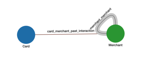 Figure 1. Merchant-to-merchant graph schema.
For the Merchant-Merchant Graph:
- Each Merchant vertex and Card vertex represents a distinct entity
- The edges card_merchant_past_interaction come directly from Card (shopper) to Merchant transactions.
- The weighted edges merchant_merchant between two Merchants represents how many common Cards are shopping between the two Merchants. These edges and their weights are not in the original data but are the result of analyzing the graph. The higher number of common Cards between two Merchants, the higher the weight and stronger the connection.
If a shopper is shopping at a given Merchant, we can use the strengths of connections to predict which other merchants they are most likely to shop at (recommendation). Or this metric can also be used as a signal for fraudulent transactions (fraud detection).
The schema for our graph looks like below where card_merchant_past_interaction edges are already available to us and we want to insert merchant_merchant edges and their corresponding weight.
Figure 2 shows an example of how merchant_merchant weighted edges would be inserted. The edge weight inserted between the two Merchants is 4 because 4 cards are in common between the two Merchants:
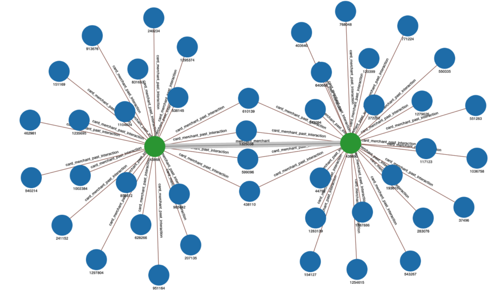
Figure 2. Example of weighted edge representing the number of common Cards between two Merchants.
2.0 Complexity Analysis and Optimization
2.1 Time Complexity of the Naive Intersection Method
To count the common neighbors (Cards in this case) between two given (Merchant) vertices A and B, we can collect the set of Card neighbors of A, those of B, and do a set intersection between the two. The time complexity for this algorithm can be determined as follows:
- Getting Neighbors for Vertex A and B: Retrieving the set of neighbors for a single vertex in an adjacency list representation of an undirected graph takes O(K) time, where K is the degree (number of incident edges) of the vertex. So, for vertices A and B it would take O(K_a + K_b) time to collect the sets of neighbors.
- Calculating Intersection: Finding the intersection of two sets with sizes n and m would generally require O(n+m) time. In our case, n=K_a and m=K_b, the number of neighbors for vertices A and B, respectively.
Time complexity for a single pair:
Combining these steps, the time complexity to calculate the Common Neighbors for a single pair of vertices (A,B) would be O(K_a + K_b).
Time complexity for all pairs:
For calculating Common Neighbors for all possible pairs of n vertices in the graph, we would need to perform this calculation n(n-1)/2 times, leading to a worst-case time complexity of O(n2K), where K is the maximum degree in the graph.
It is possible to not count intersections for all n2 pairs. To be a common neighbor, a (Card) vertex must have at least two neighbors. For each card, we can collect its list of neighboring Merchants and only continue to work with those having degree K ≥ 2. This takes O(nK) time. We only need to calculate the intersection between Merchants on these neighbor lists. The worst case length of this list would be degree K. Hence the new worst case time complexity for n vertices becomes O(nK2).
2.2 Optimized Time complexity
The optimized method aims to reduce the time complexity by altering the approach to how we count the common neighbors (or “Cards”) between two vertices (or “Merchants”) A and B. Instead of creating sets of neighbors for two merchants A and B and then finding their intersection, this method uses a direct counting approach.
Consider the Example of three Cards (C1,C2,C3) and five Merchants (M1,M2,M3,M4,M5) connected as in Figure 3:
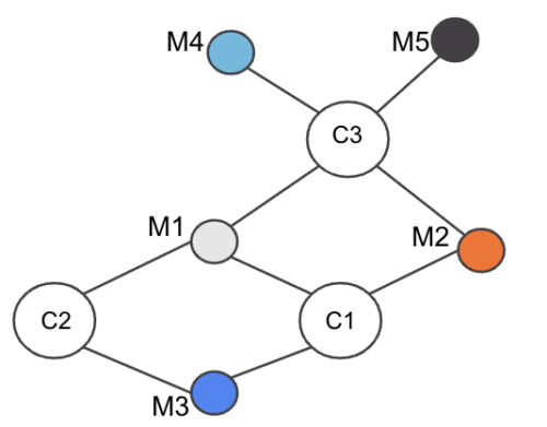
Figure 3. Merchant-Card graph example
Our objective is to find the number of common cards between each Merchant-Merchant pair.
Consider Merchant pair (M1,M3). To compute the common Cards between M1 and M3, find the set of Cards neighboring M1, i.e., S1 = {C1,C2,C3}. Next find the set of Cards neighboring M3: S2 = {C1,C2}. Now if we run the intersection , we see the set size is 2, i.e., 2 cards are common between M1 and M3. Running for all Merchant pairs M1 to M5, we can get the edge weight for all pairs of Merchants with O(nK2) complexity.
However, instead of doing intersection for each merchant pair, we can compute the edge weight using the following steps:
- Find the set of all Merchants shopped at by a Card (neighbors of the Card)
- For each Card, get each pair of Merchants in the set and do:
- Add a merchant_merchant edge if it doesn’t exist, with initial weight of 0
- Increment edge weight by 1
So for our example above in Step 1, we find all neighbors of each Card:
- C1 Set: (M1,M2,M3)
- C2 Set: (M1,M3)
- C3 Set: (M1,M2,M4,M5)
And then we iterate over each card and each Merchant pair in the set, incrementing the edge weight by 1:
- For C1 edge weight update applied:
- (M1,M2) += 1 → 1
- (M2,M3) += 1 → 1
- (M1,M3) += 1 → 1
- For C2 edge weight update applied:
- (M1,M3) += 1 → 2
- For C3 edge weights update applied:
- (M1,M2) += 1 → 2
- (M1,M4) += 1 → 1
- (M1,M5) += 1 → 1
- (M2,M4) += 1 → 1
- (M2,M5) += 1 → 1
- (M4,M5) += 1 → 1
Hence the final edge_weight pairs are as shown in Figure 4:
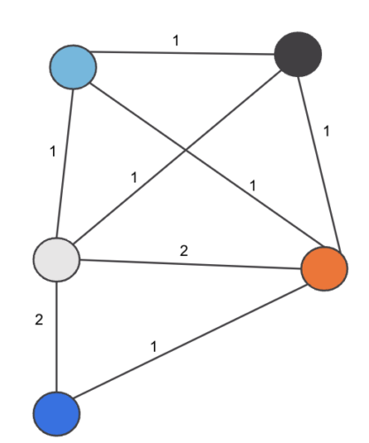
Figure 4. Weighted edges between Merchants
Hence we see from the example the time complexity can be optimized by observing the fact that we can count the number of common vertices between two vertices instead of doing an intersection and the counting operation can be done in O(1) and hence the complexity can be reduced from O(n K2) to O(nK).
3.0 Implementation in TigerGraph Using GSQL
To execute Common Neighbors algorithms, we will utilize the TigerGraph database as our graph data storage and use GSQL for algorithm implementation. Because of TigerGraph’s distributed nature we can run the algorithm distributedly and with memory efficiency.
We will evaluate performance differences between the intersect method and the optimized approach by using the above pre-established use-case: calculating common cardholders who shop at two different merchants and then assigning a weighted edge between those merchants based on that count.
The files for building Schema/Load Data and running queries in TigerGraph are in the appendix.
3.1 Intersect method GSQL implementation:
The query below shows the implementation of the Intersection method and how to insert the merchant-merchant edges in O(nK2) time.
CREATE DISTRIBUTED QUERY _02_common_cards_intersect(
  INT min_edge_weight = 1
)
FOR GRAPH optimizing_common_neighbors {
  SetAccum @merchants;
  MapAccum<VERTEX, INT> @edge_weight;
  DATETIME before;
  cards = {Card.*};
  before=(now());
  // Collect all Merchants on the Card
  merchants = SELECT m FROM cards:c- (card_merchant_past_interaction:e) - Merchant:m
              ACCUM c.@merchants+=m; //O(M) where M= number of cards
  PRINT "Time to collection of merchants on cards ",datetime_diff(now(), before);
  // INSERT edges and weights using the INTERSECT method.
  before=(now());
  temp = SELECT m FROM merchants:m -(card_merchant_past_interaction:e)- Card:c
          ACCUM
            FOREACH merc IN c.@merchants DO // O(N*K) where N =number of Merchants and K= Max degree of Card
              IF getvid(m) < getvid(merc) THEN
                tg_common_neighbors(m,merc,min_edge_weight) //O(K_a+K_b) where K_a and K_b are the degrees of the merchant pair
              END
            END; //Total complexity O(N*K*(K_a+K_b))=O(N.K^2)
  PRINT "Time to INSERT edges using intersect method",datetime_diff(now(), before);
}
The sub-query tg_common_neighbors called in the above query does the actual intersection in O(K_a + K_b) time.
Below is the sub query logic:
//Intersect subquery
CREATE QUERY tg_common_neighbors(
  VERTEX v_source,
  VERTEX v_target,
  INT min_edge_weight
)
FOR GRAPH optimizing_common_neighbors {
  avs = {v_source};
  bvs = {v_target};
  INT sz;
  na = SELECT n
       FROM avs -(card_merchant_past_interaction:e)- :n;
  nb = SELECT n
       FROM bvs -(card_merchant_past_interaction:e)- :n;
  # Get neighbors in common for source and target and compute the common neighbors
  u = na INTERSECT nb;
  sz=u.size();
  # Insert edge only if the weight is >= min_edge_weight
  IF sz >= min_edge_weight THEN
    INSERT INTO merchant_merchant (FROM ,TO ,weight) VALUES (v_source,v_target,sz) ;
  END;
}
3.2 Optimized Common Neighbors implementation
For optimization we simply replace the intersect sub query tg_common_neighbors by counting the edge weight for each merchant-merchant vertex pair and hence reduce the complexity to O(K).
CREATE DISTRIBUTED QUERY _02_common_cards_optimized(
  INT min_edge_weight = 1
)
FOR GRAPH optimizing_common_neighbors {
  SetAccum @merchants;
  MapAccum<VERTEX, INT> @edge_weight;
  DATETIME before;
  cards = {Card.*};
  before=(now());
  // Collect all Merchants on the Card
  merchants = SELECT m FROM cards:c- (card_merchant_past_interaction:e) - Merchant:m
              ACCUM c.@merchants+=m; //O(M) where M= number of cards
  PRINT "Time to collection of merchants on cards ",datetime_diff(now(), before);
  // Establish logical edges an summed weights
  before=(now());
  temp = SELECT m FROM merchants:m -(card_merchant_past_interaction:e)- Card:c
          ACCUM
            FOREACH merc IN c.@merchants DO // O(N*K) where N =number of Merchants and K= Max degree of Card
              IF getvid(m) < getvid(merc) THEN m.@edge_weight += (merc -> 1) //O(1)
              END
            END; //Total complexity O(N*K*1)=O(N.K)
  PRINT "Time to establish merchant-merchant edges using optimized common neighbors ",datetime_diff(now(), before);
  // Insert edges
  before=(now());
  temp = SELECT m FROM merchants:m
          POST-ACCUM
            FOREACH (merc, w) IN m.@edge_weight DO
              IF w >= min_edge_weight THEN                 // Insert edge only if the weight is >= min_edge_weight
                  INSERT INTO merchant_merchant VALUES (m, merc, w)
              END
            END;
  PRINT "Time to INSERT merchant-merchant edges  ",datetime_diff(now(), before);
}
4. Performance Comparison
For comparing the performance of the two algorithms the data metrics and hardware being used are as follows:
Data Metrics:
| Metric | Count |
| All Vertices | 1,807,672 |
| All Edges | 6,872,163 |
| Vertex “Card” | 1,335,486 |
| Vertex “Merchant” | 472,186 |
| Edge “card_merchant_past_interaction” | 6,872,163 |
| Edge “merchant_merchant” | 0 |
Raw Data size = 95.1MB.
The final count of “merchant_merchant” edges inserted is 20,607,316.
Hardware Configuration:
2 x TG.C16.M64 TigerGraph Cloud instances (16 CPUs, 64GB Memory)
The following Table captures the performance of the two algorithms.
| Metric | Intersection Method | Optimized Method | Notes |
| Execution Time (Seconds) | 3517.49 | 23.33 | 153x Speed improvement |
| Peak Memory Usage (GB) | 8.1 | 2.1 | 4x Memory reduction |
Lorem ipsum dolor sit amet, consectetur adipiscing elit. Ut elit tellus, luctus nec ullamcorper mattis, pulvinar dapibus leo.
5.0 Conclusion
The optimized algorithm significantly outperforms the intersection-based approach, not just in speed but also in memory efficiency. TigerGraph’s GSQL enables users to tailor algorithms to their specific needs, offering unparalleled flexibility and scalability. For additional examples of graph algorithms implemented in GSQL, please refer to our Graph Data Science Library.
Appendix
Solution that can be run in GSQL shell
Notebook to create Schema/Load_data/install queries
Graph Data File for Card-Merchant Edges
If you’re interested in exploring how TigerGraph can open up new dimensions with your data, you can sign up for a free instance of TigerGraph Cloud at tgcloud.io or contact us at info@tigergraph.abstage.xyz.